A Maxima tutorial

1 Introduction

Maxima is a Free Software package for the manipulation of symbolic and numerical expressions, including differentiation, integration, Taylor series, Laplace transforms, ordinary differential equations, systems of linear equations, polynomials, sets, lists, vectors, matrices and tensors and more. It can be freely downloaded from its Website (https://maxima.sourceforge.net) which also includes reference manuals and tutorials in several languages. There is an active community of developers and users; questions about Maxima can be sent to its main mailing-list address at maxima-discuss@lists.sourceforge.net.

Maxima is one of the oldest Computer Algebra Systems (CAS). It was created by MIT's MAC group in the 1960s and it was initially called Macsyma (project MAC's SYmbolic MAnipulator). Macsyma was originally developed for the DEC-PDP-10 large-scale computers that were used in various academic institutions at that time.

In the 1980s, its code was ported to several new platforms and one of those derived versions was called Maxima. In 1982 the MIT decided to sell Macsyma as proprietary software and simultaneously Professor William Schelter of the University of Texas continued to develop the Maxima version. In the late 1980s other proprietary CAS systems similar to Macsyma appeared, such as Maple and Mathematica. In 1998, Professor Schelter obtained authorization from the DOE (Department of Energy), which held the copyright for the original version of Macsyma, to distribute the source code of Maxima as free software. When Professor Schelter passed away in 2001, a group of volunteers was formed to continue to develop and distribute Maxima as free software.

In the case of CAS software, the advantages of free software are very important. When a method fails or gives very complicated answers it is quite useful to have access to the details of the underlying implementation of the methods used. On the other hand, as one's research and teaching becomes dependent on the results of a CAS, it is desirable to have good documentation of the methods involved and its implementation and to be assured that there are no legal barriers forbidding the examination and modification of that code.

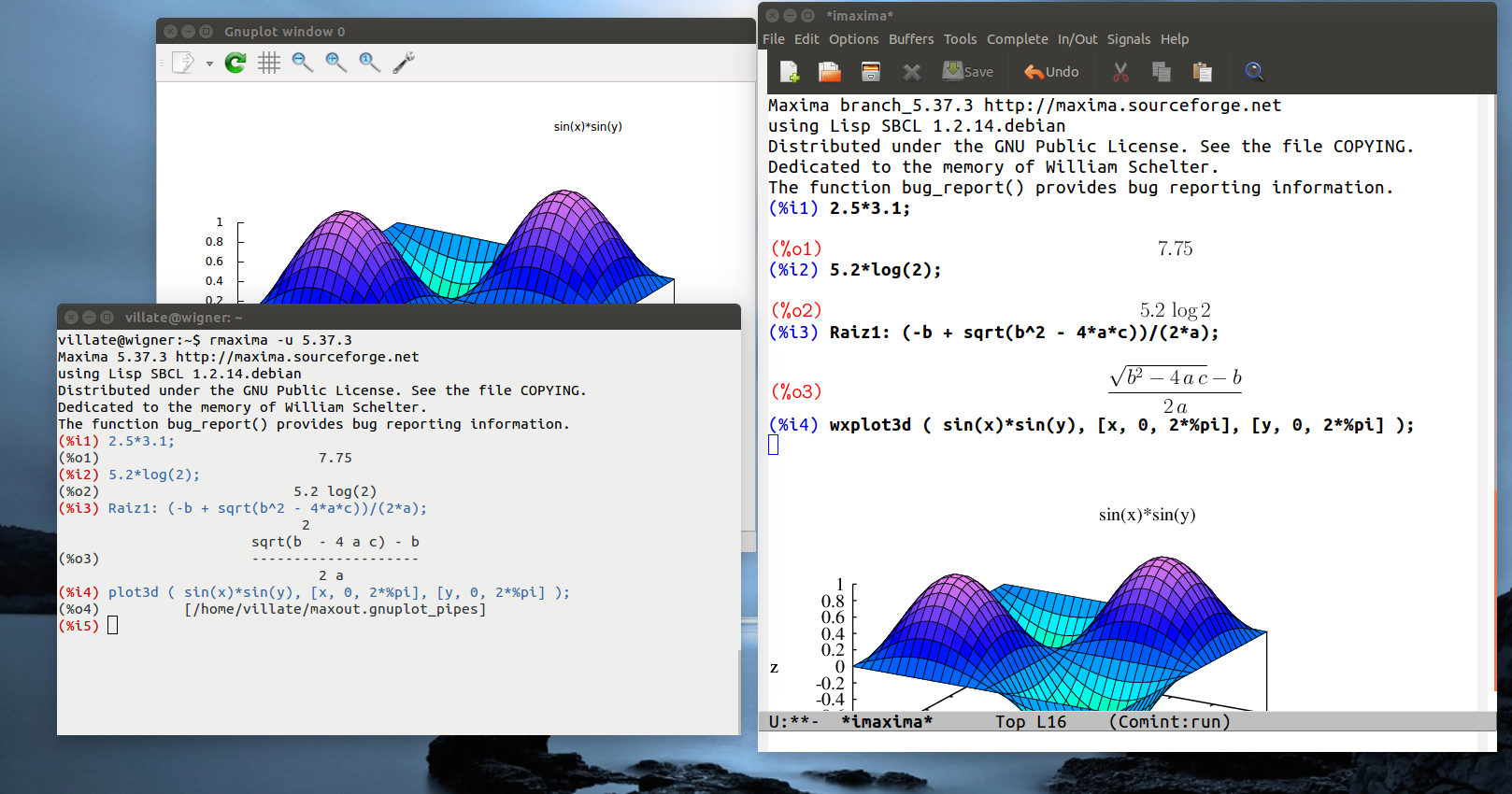
2 Graphical interfaces for maxima

Maxima is a program that uses a command shell (or a console or text terminal) to interact with the user. There are also several graphical interfaces to work with Maxima, such as wxMaxima, which is a software package separate from Maxima; you might have to install that package separately, if it's not bundled to the package you download to install Maxima. Two other graphical interfaces, imaxima and Xmaxima, are being developed and distributed together with Maxima. The left-hand side of Figure 1 shows some commands being run in Xmaxima, and the right-hand side shows the same commands as being run in imaxima, which runs from within the Emacs text editor

**Figure 1:** Xmaxima's graphical interface.

The graphical interfaces connect to the Maxima program, send the commands that the user types to Maxima, and show the result it returns. Some interfaces, such as wxMaxima and imaxima, convert those results to a graphic that resembles closer what the user would find in a textbook, while Xmaxima leaves the result as given by Maxima, namely simple text that can take several lines in the case of fractions, powers or long output.

Xmaxima usually opens two windows (Figure 1). One of them, called the browser, shows a tutorial and allows the user to read the manual or other Web pages. The second window is the console, where Maxima commands should be written and their output will appear.

In the "Edit" menu there are options to navigate the list of previous commands ("previous input") or to copy and paste text; some options in the menus can also be accessed with the shortcut keys shown next to them. Different colors are used to distinguish commands that have already been processed (in blue) from the command that is being written and has not yet been sent to Maxima (in green); the results are shown in black (see Figure 1).

When changing a command already executed or when starting a new command, care must be taken that what is being written appears in green or blue, to ensure that it will be sent to Maxima. Sometimes it may be necessary to use the options "Interrupt" or "Input prompt", in the "File" menu to recover the state in which Xmaxima is accepting commands.

It is also possible to move the prompt symbol to some older entry in the screen (in blue), change it, and press enter to repeat the same command with the modifications.

3 Data input and output

When a Maxima session starts, the tag (%i1) will appear, which refers to input 1. A valid command should be written next to that tag, ended with a semi-colon and when the enter key is pressed, that input will be parsed, simplified, linked to an internal variable %i1 and its result will be shown following a tag (%o1), referring to output 1. That result will also be linked to an internal variable %o1. Another tag (%i2) will then appear, to mark the place where a second command may be written and so on. The most basic usage of Maxima is as a calculator, as in the following examples.

(%i1) 2.5*3.1;
    
(%o1)                           7.75
    
(%i2) 5.2*log(2);
    
(%o2)                        5.2 log(2)

The result in %o2 shows two important aspects of Maxima. First, the natural logarithm of 2 was not computed, because its result is an irrational number which cannot be represented exactly with a finite number of numerical digits. The second important aspect is that the symbol * which is always required when a product is entered and the parenthesis, which have to be used to specify the argument of a function, were not included in the output. That happened because, by default, the output is shown in a mode called display2d, in which the output tries to resemble the way mathematical expressions are usually shown in books. The expression "5.2 log 2" most probably will be interpreted correctly by a reader, as the product of 5.2 times the logarithm of 2; however, if that same ambiguous expression was given as input to Maxima it would trigger an error, because Maxima syntax requires an operator between 5.2 and the logarithm function, and the argument of the logarithm must be inside parenthesis. In spite of the form of the output, variable %o2 has been linked to an expression with correct syntax, so it can be reused in later Maxima commands without syntax errors.

To look up the documentation of a function or special variable in the manual, for instance the function log that was just used, the describe function is used, which can be abbreviated with a question mark followed by space and the name of the function:

(%i3) ? linel;

 -- Option variable: linel
     Default value: '79'

     'linel' is the assumed width (in characters) of the console display
     for the purpose of displaying expressions.  'linel' may be assigned
     any value by the user, although very small or very large values may
     be impractical.  Text printed by built-in Maxima functions, such as
     error messages and the output of 'describe', is not affected by
     'linel'.

  There are also some inexact matches for `linel'.
  Try `?? linel' to see them.

(%o3)                             true

4 Numbers

Maxima accepts real and complex numbers. Real numbers in Maxima can be integers, rationals, such as 3/5, or floating-point numbers, for instance, 2.56 and 25.6e-1, which is a short notation for $25.6 \times 10^{- 1}$ . Irrational numbers, such as sqrt(2) or log(2) (natural logarithm of 2) are left in that form, without being approximated by floating-point numbers, and later calculations, such as sqrt(2)*sqrt(2) or exp(log(2)) will lead to the exact result 2.

Floating-point numbers are "contagious"; namely, the operations in which they enter will be carried out in that format. For example, if instead of writing log(2) we would write log(2.0), the logarithm would be computed approximately in floating-point. Another way to force an expression to be computed as a floating-point number consists on using the function float. For instance, since the result (%o2) above has been stored in variable %o2, to get a floating-point approximation of that result we would write:

(%i4) float (%o2);

(%o4)                    3.6043653389117156

The function float computed the product $5.2 \log (2)$ approximately, using 16 significant digits in floating-point format. The floating-point format used in Maxima stores each number in 64 binary bits, which leads to between 15 and 17 significant digits when expressed in decimal base. That format is known as double precision.

A frequent source of confusion arises from the fact that those numbers are being represented internally in binary base and not in decimal base; thus, certain numbers that can be represented in decimal base with a few digits, for instance 0.1, would need an infinite number of binary digits to be represented accurately in binary base. It is the situation as with the fraction 1/3 in decimal base, which in floating-point form has an infinite number of digits: 0.333…, while in base 3 that fraction would simply be 0.1.

The fractions that lead to an infinite number of digits are not the same in the decimal and binary base. Consider the following results, which would appear in any system that uses binary base and double-precision format and which might puzzle somebody used to working with in decimal base:

(%i5) 2*0.1;

(%o5)                           0.2

(%i6) 6*0.1;

(%o6)                    0.6000000000000001

Some computing systems ignore the last digits in the results obtained from double-precision calculations, showing the result as 0.6, but whenever binary double-precision is used, the result of 6×0.1 will not be exactly 0.6.

The best approximation of 1/3 in decimal base, using only 3 significant digits, is $333 / 10^{3} = 0.333$ . In binary base, it is represented as $n / 2^{m}$ ( $n$ and $m$ integers); with the 52 significant digits used in the double-precision standard, $n$ has to be less than $2^{52}$ . Maxima's function rationalize shows the approximate representation being used for a number, in the form of a fraction. For instance the approximation to $0.1$ is

(%i7) rationalize (0.1);

                         3602879701896397
(%o7)                    ─────────────────
                         36028797018963968

where 3602879701896397 is less than $2^{52}$ and bigger than $2^{51}$ , and the denominator is a power of 2 ( $36028797018963968 = 2^{55}$ ). That fraction is not exactly equal to $0.1$ , but it is the best possible approximation using double-precision.

There is a Maxima specific format which accepts bigger number of significant digits to represent floating-point numbers, called bigfloat. To use it, one should write "b", instead of "e" for the exponents; for example, $2.56 \times 10^{20}$ , written as 2.56e20 would be represented internally in double-precision format, with 16 significant digits, and any calculations made with it would result in other double-precision numbers. But if the same number was written as 2.56b20, it would be stored in the bigfloat format and any calculations involving it would produce other bogfloat numbers. By default, bigfloat format uses the same 16 significant digits as double-precision, but that can be changed by changing the value of the system variable fpprec (floating-point precision).

Function bfloat converts a number into bigfloat. For example, to show an approximation to the result save in variable %o2 with 60 significant digits, the following commands can be used:

(%i8) fpprec: 60;

(%o8)                            60

(%i9) bfloat (%o2);

(%o9) 
     3.60436533891171573209728052144843624984298344312084369367127b0

The letter b followed by zero at the end of (%o9) means that the number is stored in bigfloat format and it should be multiplied by a factor of $10^{0} = 1$ .

In the rest of this tutorial we will show all floating-point results with only 4 significant digits. That is achieved by changing system variable fpprintprec from its default value of 0 to 4:

(%i10) fpprintprec: 4;

(%o10)                           4

Internally, all floating-point double-precision numbers will continue to have 16 significant digits and bigfloat numbers will have the number of significant digits set by fpprec, but whenever a number has to be printed in the screen, it will be rounded to 4 significant digits. If we would like to see all the significant digits stored internally, variable fpprintprec should be set to its default value of 0.

5 Variables

To bind a numerical value or other objects to a variable, we use a colon ":" and not the equal sign "=" which is reserved to define mathematical equations. The name of the variables can be any combination of letters, numbers and the characters % and _, but the first character cannot be a number. Maxima is case sensitive. Here are some examples:

(%i11) a: 2$

(%i12) [b, c]: [-2, -4];

(%o12)                       [- 2, - 4]

(%i13) c;

(%o13)                          - 4

(%i14) Root1: (-b + sqrt(b^2 - 4*a*c))/(2*a);

(%o14)                           2

(%i15) d: sqrt(z^2 + a*c);

                                   2
(%o15)                      sqrt(z  - 8)

variables a, b, c and Root1 were bound to the numerical values 2, $- 2$ , $- 4$ and 2, while variable d was bound to an expression.

Notice that input (%i11) was ended with a dollar sign $, rather than a semi-colon. That will make the command to be executed without showing its result on the screen. In spite of not being displayed on the screen, that result has been bound to the symbol %o11 so it can be used later on.

Input (%i12) shows how to bind several variables to several values with a single command. When the name of a variable is written, as in input (%i13), the output will be the value bound to that variable or the name of the variable itself if it has not been bound to any value. In (%i14), the values bound to a, b and c were replaced and the result was bound to variable Root1. If the values bound to a, b or c are later changed, that will not affect the value already bound to Root1.

In (%i15) since z has not yet been bound to any value, it is just a symbol and variable d is then bound to an expression that depends on that symbol. Variables can be bound to numerical values, expressions with abstract symbols, equations and several other objects that will be described in the following sections. That means that when you add two variables, you could be adding a mix of numbers, expressions, equations and so on; the result could lead to some other valid object or to an error it Maxima can not sum those objects.

To remove the value bound to a variable, the function remvalue can be used; in the following example the value bound to a is removed and an expression that depends on the symbol a is then bound to Root1:

(%i16) remvalue (a)$

(%i17) Root1: (-b + sqrt(b^2 - 4*a*c))/(2*a);

                         sqrt(16 a + 4) + 2
(%o17)                   ──────────────────
                                2 a

The command remvalue(all) removes all values bound to variables

The following 2 commands will show the value obtained from the expression bound to Root1, when a is replaced by 1 and the result is approximated to a floating-point number.

(%i18) subst (a=1, Root1);

                           2 sqrt(5) + 2
(%o18)                     ─────────────
                                 2

(%i19) float(%o18);

(%o19)                         3.236

The objects associated to a and Root1 are not modified after (%i18); a continues to be an abstract symbol and Root1 is associated to an expression that depends on the symbol a.

Maxima uses several system variables, whose names start by %. Some examples are the variables %i2 and %o2, linked to an input command and its result. The character % itself represents the last result obtained. For instance, in (%i19) it would have been enough to write down % instead of %o18. The two commands (%i18) and (%i19) could have been combined into a single command float (subst (a=1, Root1)).

A variable can also be associated to an algebraic equation, as in the following example

(%i20) second_law: F = m*a;

(%o20)                        F = a m

Maxima does some simplifications to the input commands before executing them. In this last example, the result of that simplification was to change the order of the product, to put the two symbols in alphabetical order. If any of the 3 symbols F, m or a were associated to a value or other object, that object would have been substituted by the simplifier. To prevent the value of a variable to be replaced, its name can be preceded by an apostrophe ('a refers to the symbol a and not to any object associated to it).

The following example shows how the equation associated to second_law does not change when one of the symbols in it s then associated to a value

(%i21) a: 3;

(%o21)                           3

(%i22) second_law;

(%o22)                        F = a m

The function subst is used to substitute values of the symbols in second_law. Several values can be replaced at once, as in the following example

(%i23) subst([m=2,'a=5], second_law);

(%o23)                         F = 10

The first argument in the subst command in (%i23) is a list, whose elements are separated by commas and within square brackets. The two elements in that list are equations. In the second equation 'a was quoted to prevent it from being replaced by the value 3 associated to symbol a. Without the quote, the subst command would have been simplified as

(%i24) subst([m=2, 3=5], second_law);

(%o24)                        F = 2 a

and then only m is replaced and the statement "3=5" is simply ignored because it does not name any variable in the expression where the substitution is done.

6 Lists

As seen in the previous section, lists can be created using square brackets and commas. The following example creates a list with the squares of the first five natural numbers and associates it to the variable squares

(%i25) squares: [1, 4, 9, 16, 25]$

Many of the operations among numbers can also be done among lists. For example, let us create another list in which each element is the square root of the corresponding element of squares, multiplied by 3

(%i26) 3*sqrt(squares);

(%o26)                   [3, 6, 9, 12, 15]

The elements of a list are indexed by integers starting with 1. To refer to an element in the list, the corresponding index is written within square brackets; for instance the third element in the list squares is

(%i27) squares[3];

(%o27)                           9

A very useful function to create lists is makelist. One way to use it is to expand an expression depending on a dummy index, for several values of that index. The first argument must be the expression to be expanded, followed by the dummy index, the initial value for it, the upper bound for the index values and the increments between successive values of the index. If the increment is not given, its default value is 1. Here are two examples:

(%i28) cubes1: makelist ( i^3, i, 1, 5 );

(%o28)                  [1, 8, 27, 64, 125]

(%i29) cubes2: makelist ( i^3, i, 2, 6, 0.6);

(%o29)     [8, 17.58, 32.77, 54.87, 85.18, 125.0, 175.6]

The first list has the cubes of 1, 2, 3, 4 and 5. The second one has the cubes of 2, 2.6, 3.2, 3.8, 4.4, 5.0 and 5.6. Notice that the elements of cubes2 are shown with only 4 significant digits, because in (%i10) we changed the value of the system variable fpprintprec. In a fresh Maxima session they would be shown with 16 significant digits.

Instead of giving an initial value and an upper bound for the dummy index, we can give a list of values for it. And that list can have objects of different types. The following example creates a list with the cubes of 5, the expression $x^{2} + \sqrt{y}$ , $- 3.2$ (in bigfloat format) and the equation $E = m c^{2}$

(%i30) makelist (i^3, i, [5, x^2+sqrt(y), -3.2b0, E=m*c^2]);

                            2 3              3         3
(%o30)    [125, (sqrt(y) + x ) , - 3.277b1, E  = 4096 m ]

8 Batch files

The command stringout("filename",input) will store all the input commands that have been entered during a Maxima session, into a file named "filename". That file can be loaded in a future Maxima session, to redo all those commands, with the command batch("filename"). The name of Maxima batch files are usually given the extension .mac to identify them as Maxima batch files.

You can also create a Maxima batch file with a text editor. Just write the input commands (without any %i labels) and then execute it in Maxima with batch("filename"). That is a useful way to use Maxima to solve a problem. You write your commands to solve the problem in a text editor, save them into a file, and without closing the editor open Maxima in another window and run that file. If there is an error or you don't get the result you wanted, you just have to go back to the editor window, make the necessary modifications, save them and back in the Maxima window rerun the batch file. Be careful not to use %o variables in batch files, because the number after %o might be different every time you execute them.

Many additional functionalities of Maxima come into batch files which you execute in Maxima using load("filename"). The difference between batch and load is that load will not show the result of the commands being executed. Both commands have a predefined list of directories where they will look for the file with name "filename".

Batch files can include any comments, opening with the two characters /* and closing with */. Any commands entered directly into Maxima or written into a batch file can contain blank spaces and new lines between numbers, operators, variables and other objects, in order to make them more readable.

Some commands that are used repeatedly in different working sessions, for instance, the definition a frequently used function, can be placed inside a batch file which can be loaded in future sessions. If the name of a batch file to be loaded does not include a complete path but just the file name and that file name does not exist in the current directory, Maxima will look for it in a set of directories. That set of directories includes a sub-directory of the users home directory. The name of that sub-directory can be different in different systems but it is always stored in Maxima's system variable maxima_userdir. You can look at the value of that variable and if the referred sub-directory does not exist, created them. Any batch files you put into that sub-directory can then be loaded into Maxima by giving its name, independently of the working directory being used in the current Maxima session.

Every time Maxima starts it tries to load a user's batch file in that maxima_userdir, with the name maxima-init.mac, before showing the first input prompt. That means that you can create that file, if it doesn't already exist, and add commands that you want to be used in all your Maxima sessions. For example, the contents of file maxima-init.mac could be the following

ratprint: false$
  
linel: 66$

The first command prevents Maxima from showing warning messages every time a floating-point number is replaced by a fraction, something many Maxima functions do, and the second command limits the maximum length of output lines to 66 characters. In a Linux system that file would be located in /home/username/.maxima/ and in Windows, in a folder maxima within the user's directory.

Any other valid Maxima commands can be placed into that file, but keep in mind that if any of those commands fail, the error might prevent Maxima from starting until that initial batch file is corrected.

9 Algebra

Expressions can include mathematical functions, such as the function cosine in the following example

(%i33) 3*x^2 + 2*cos(t)$

Those expressions can then be manipulated producing new expressions. In the next example we find the square of the expression above and add $x^{3}$ to it

(%i34) %^2 + x^3;

                          2            2    3
(%o34)                (3 x  + 2 cos(t))  + x

As we have already mentioned besides numbers and expressions, other kind of object we can manipulate is an equation as the following one

(%i35) 3*x^3 + 5*x^2 = x - 6;

                           3      2
(%o35)                  3 x  + 5 x  = x - 6

Most functions used to manipulate expressions can also be used for equations. For example, Maxima's function allroots finds a numerical approximation to the roots of a polynomial, such as $x^{2} + x - 1$ ; if allroots is given the equation $x^{2} + x = 1$ , it will interpreted as $x^{2} + x - 1 = 0$ and find the roots of $x^{2} + x - 1$ . Therefore, when given the expression in %o35, allroots will find the roots of $3 x^{3} + 5 x - x + 6$

(%i36) allroots(%o35);

(%o36) [x = 0.9073 %i + 0.2776, x = 0.2776 - 0.9073 %i, x = - 2.222]

Two of those roots are complex numbers. The three roots are shown as a list of three equations, instead of just numbers. That way of presenting the result may seem odd, but it will prove convenient to interact with other functions of Maxima. For example, to check that the third root shown is in fact a root of the polynomial $3 x^{3} + 5 x - x + 6$ , we write

(%i37) subst(%o36[3], 3*x^3+5*x^2-x+6);

(%o39)                       7.105e-15

The notation %o36[3] means the third element in the list associated to variable %o36, which is the equation $x = - 2.222$ and it is exactly what we need to tell subst to substitute $x$ by $- 2.222$ . It is in fact substituted to by $- 2.221834293486762$ which is the value stored in list %o36; the output (%o36) is the exact result rounded to 4 significant digits, since set the number of displayed digits for floating-point numbers equal to 4 in (%i10). The floating-point values in the list bound to %o36 all have approximately 16 digits (the default for double-precision binary numbers). The result (%o37) is not zero, because allroots is a numerical algorithm and its results have a numerical error which in double-precision is of the order of $10^{- 15}$ .

There are other functions to find the exact solution to an algebraic equation without numerical approximations. Function solve can find the exact solutions to some algebraic equations or systems of algebraic equations (see the documentation for solve if you would like to know the type of equations that it can solve). In the case of equation (%o35), the exact algebraic expressions for the three solutions in %o36 can be found with:

(%i38) result: solve ( 3*x^3 + 2*x^2 = x - 6, x )$

Since the result is very lengthy, we didn't show it on the screen but saved it into the list result. The third root is the 3 element of that list, which can be written in a simpler form using one of the simplifying functions for algebraic equations. In the next 3 commands we will use three of those simplifying functions.

(%i39) factor (result[3]);

                                         2/3
(%o39) x = ((27 sqrt(2393) - 764 sqrt(3))
      1/6                              1/3       1/3
 - 2 3    (27 sqrt(2393) - 764 sqrt(3))    + 13 3   )
   13/6                              1/3
/(3     (27 sqrt(2393) - 764 sqrt(3))   )

(%i40) xthru (result[3]);

(%o40) x = 
        5/2                  2/3       5/2                  1/3
      (3    sqrt(2393) - 764)    - 2 (3    sqrt(2393) - 764)    + 13
      ──────────────────────────────────────────────────────────────
                           5/2                  1/3
                       9 (3    sqrt(2393) - 764)

(%i41) ratsimp (result[3]);

                                         2/3
(%o41) x = ((27 sqrt(2393) - 764 sqrt(3))
      1/6                              1/3       1/3
 - 2 3    (27 sqrt(2393) - 764 sqrt(3))    + 13 3   )
   13/6                              1/3
/(3     (27 sqrt(2393) - 764 sqrt(3))   )

Which of the 3 previous expressions is simpler is just a matter of taste; they are all equivalent. Thus, when simplifying algebraic results you should try with those different functions and choose the result that you like the most. In this case functions ratsimp and factor gave the same result, but in other cases they might give different results. There are other simplifying functions; one that is also used often is radcan.

You can also try to look at the two complex roots in result, using function rectform to separate the real and imaginary parts.

Systems of linear equations and some nonlinear systems can also be solved using solve. The two equations must be given into a list, as in the following example

(%i42) exp1: (4 + 8)*x1 - 8* x2 = 6 + 4$

(%i43) exp2: (2 + 8 + 5 + 1)*x2 - 8*x1 = -4$

(%i44) solve ( [exp1, exp2], [x1, x2] );

                                        1
(%o44)                   [[x1 = 1, x2 = ─]]
                                        4

There are two features of solve involved in the previous example. First, instead of 2 equations, we provided two expressions; every expression given to solve is then interpreted as that expression being equal to zero. Second, there is an optional argument, after the equations, with the variable or list of variables to be solved; if given, the number of variables must be equal to the number of equations. In the examples we have given there is no need to name the variables, because those variables are the only ones that appear in the equations. However, in some cases the name of the variables is necessary; for instance to solve just one equation $x / y^{2} = \sqrt{z}$ with three variables, we must specify what variable we want to get in terms of the other two.

The result saved in variable %o44 is a list of solutions, where each possible solution is represented by a list. In this case there is only one solution which then appears as a list within another list.

Function expand will expand products and powers of expressions, as in the following example

(%i45) expand ((4*x^2*y + 2*y^2)^3);

                  6       2  5       4  4       6  3
(%o45)         8 y  + 48 x  y  + 96 x  y  + 64 x  y

Function subst, which we used before to substitute numerical values, can also be used to substitute other expressions. In the next example we substitute $x$ by $1 / z$ , and $y$ by $\sqrt{z}$ in the expression %o43:

(%i46) subst([x=1/z, y=sqrt(z)], %o43);

(%o46)                   16 x2 - 8 x1 = - 4

We can save that result into a variable, for instance r

(%i47) r: %$

Algebraic expressions are represented internally as lists; hence, some Maxima functions for lists can also be used with expressions. For instance, function length gives the length of a list and it can also be used to compute the number of terms in an expression; for instance,

(%i48) length(r);

(%o48)                             2

Since the expression r was combined into a single fraction, the corresponding list has two elements, the numerator and denominator of that fraction. However, the two elements of the expression cannot be obtained with r[1] and r[2] as we have previously done with regular lists. In this case we have to use the functions first and second. The following command shows the numerator of r

(%i49) first(r);

(%o49)                        16 x2 - 8 x1

and the length of that expression is

(%i50) length(%);

(%o50)                             2

because it is the sum of three other expressions.

A Maxima expression that cannot be further separated into other sub-expressions, for instance $x$ or $- 3.5$ , is dubbed an atom; functions that expect a list as its argument will usually trigger an error when they are given an atom as the argument. Function atom tells whether the argument given is an atom or not.

A very useful function to manipulate lists or expressions is map, which will apply a given function to each element in a list. Here is an example: suppose we have the following expression, which we will save into a variable f

(%i51) f: (x+y)^2 / (x-y)^2;

                                       2
                                (y + x)
(%o51)                          ────────
                                       2
                                (x - y)

We now would like to expand the squares in the numerator and denominator, but if we try to expand f, the result is the following

(%i52) expand (f);

                 2                                   2
                y                2 x y              x
(%o52)    ─────────────── + ─────────────── + ───────────────
           2            2    2            2    2            2
          y  - 2 x y + x    y  - 2 x y + x    y  - 2 x y + x

The fraction was also expanded into 3 other fractions, which is not what we wanted. If we map expand to the two terms of the fraction, the numerator and denominator will be expanded separately giving the following result

(%i53) map (expand, f);

                             2            2
                            y  + 2 x y + x
(%o53)                      ───────────────
                             2            2
                            y  - 2 x y + x

11 Trigonometry

Table 1 shows the names of the main trigonometric functions in Maxima. Angles are given in radians, and not in degrees.

When applied to a floating-point number, these functions will give another floating-point number. But if the argument is not a floating-point number, the result is simplified but not computed, unless for some known numbers for which the exact result is known, as in the following example. Function float can be used to get an approximate floating-point result

(%i55) [sin(-0.5), cos(-1/2), tan(%pi/3)];

                                     1
(%o55)                [- 0.4794, cos(─), sqrt(3)]
                                     2


(%i56) float(%);

(%o56)                 [- 0.4794, 0.8776, 1.732]

Consider the point with $x$ coordinate $- 1$ and $y$ coordinate 1; the position vector of that point makes an angle of $3 π / 4$ radians with the x-axis, and the tangent of that angle is $- 1$ but if one computes atan(-1), the result would be $- π / 4$ because arc tangent has many branches and the branch chosen in Maxima goes from $- π / 2$ to $π / 2$ . The $y$ and $x$ coordinates can be given to function atan2 and it will compute the correct angle:

(%i57) atan2(1, -1);

                                 3 %pi
(%o57)                           ─────
                                   4

To convert an angle from degrees into radians, it is multiplied by $π$ and divided by 180. In the following example we compute the sine of $60^{\circ}$

(%i58) sin(60*%pi/180);

                                sqrt(3)
(%o58)                          ───────
                                   2

and to convert the results of the arc functions from radians to degrees, they should be multiplied by 180 and divided by $π$ .

There are some functions that simplify trigonometric expressions. Function trigexpand expands sines and cosines of sums of angles:

(%i59) trigexpand(sin(u+v)*cos(u)^3);

                   3
(%o59)          cos (u) (cos(u) sin(v) + sin(u) cos(v))

And function trigreduce tries to convert an expression into a sum of terms with a single trigonometric function:

(%i60) trigreduce(%);

        sin(v + 4 u) + sin(v - 2 u)   3 sin(v + 2 u) + 3 sin(v)
(%o60)  ─────────────────────────── + ─────────────────────────
                     8                            8

Function trigsimp applies the trigonometric identity $\sin^{2} x + \cos^{2} x = 1$ and relations among trigonometric functions, trying to write the expression using only sines and cosines, as in the following example

(%i61) tan(x)*sec(x)^2 + cos(x)*(1 - sin(x)^2);

                    2                            2
(%o61)           sec (x) tan(x) + cos(x) (1 - sin (x))


(%i62) trigsimp(%);

                                        6
                            sin(x) + cos (x)
(%o62)                      ────────────────
                                   3
                                cos (x)

12 Calculus

The simplest way to represent mathematical functions in Maxima is by using expressions. For example, to represent function $f (x) = 3 x^{2} - 5 x$ , the expression on the right-hand-side is linked to variable $f$

(%i63) f: 3*x^2 - 5*x;

                                  2
(%o63)                         3 x  - 5 x

The derivative of $f$ with respect to $x$ is computed using function diff

(%i64) diff (f, x);

(%o64)                          6 x - 5

and the antiderivative with respect to $x$ is obtained with integrate

(%i65) integrate (f, x);

                                       2
                                3   5 x
(%o65)                         x  - ────
                                     2

The value of the function at a point, for instance $f (1)$ , can be obtained substituting $x$ by 1 using subst, or with function at

(%i66) at (f, x=1);

(%o66)                            - 2

Maxima also has its own syntax to define general functions, which is the subject of a later section, and which can be used when the function's result is an expression. For example, the same function $f (x) = 3 x^{2} - 5 x$ could have also be defined as follows

(%i67) f(x) := 3*x^2 - 5*x;

                                      2
(%o67)                     f(x) := 3 x  - 5 x

The value of the function at a point, for instance $x = 1$ , and the function's derivative and antiderivative could then be obtained in this way

(%i68) f(1);

(%o68)                            - 2


(%i69) diff (f(x), x);

(%o69)                          6 x - 5


(%i70) integrate (f(x), x);

                                       2
                                3   5 x
(%o70)                         x  - ────
                                     2

Notice that in (%i66) and (%67) Maxima would first get the output of function $f$ when the its input is $x$ , leading to the result $3 x^{2} - 5 x$ and then the derivative or antiderivative are computed. Therefore, (%i66) does not really differentiate Maxima's function $f$ , but rather the expression associated to it. And similarly in (%67)

When the output of Maxima's function $f (x)$ is not an expression, (or a list of expressions), diff and integrate return the result of $f (x)$ without being differentiated or integrate, as in the following example

(%i71) h(x) := if x < 0 then x/2 else x^2;

                                          x       2
(%o71)              h(x) := if x < 0 then ─ else x
                                          2

(%i72) diff (h(x), x);

                      d                 x       2
(%o72)                ── (if x < 0 then ─ else x )
                      dx                2

When given an expression with several variables, diff returns a partial derivative with respect to the differentiating variable and integrate assumes constant values for the variables not being integrated

(%i73) diff (x^2*y-y^3, x);

(%o73)                           2 x y

Function integrate can also be used to computed definite integrals, as in the following example

(%i74) integrate (1/(1 + x^2), x, 0, 1);

                                  %pi
(%o74)                            ───
                                   4

13 Plots

The function plot2d is used to plot curves or points in two dimensions. For example, the plot of the polynomial $t^{3} + t^{2} - 2 t$ , for values of $t$ between $- 3$ and $2$ , can be done with the following command

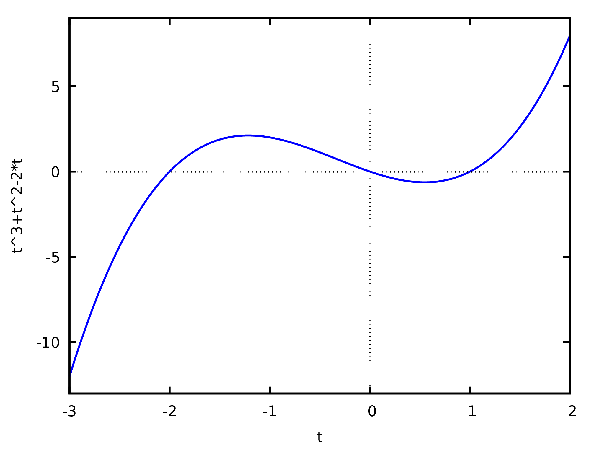
(%i75) plot2d (t^3+t^2-2*t,[t,-3,2])$

**Figure 2:** Plot of the polynomial $t^{3} + t^{2} - 2 t$ .

The result of (%i74), shown in Figure 2, will appear in a separate window. Moving the mouse over the plot, the coordinates of the point where the cursor is are shown.

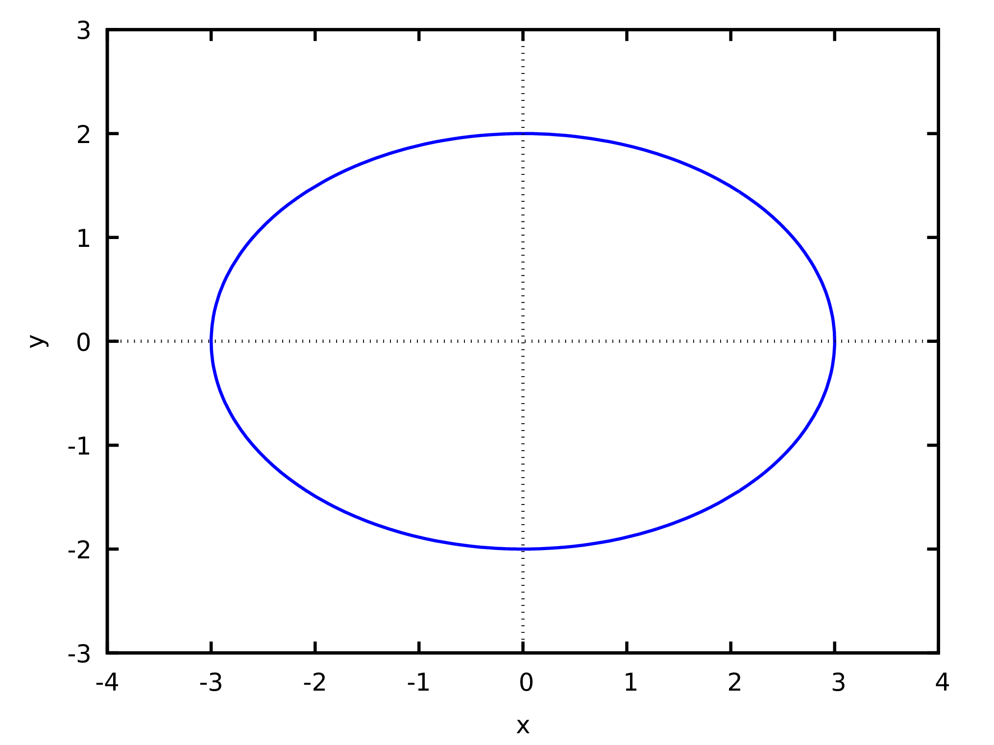
The expression to plot can also be an equation with 2 variables. In that case it is necessary to give ranges of values for those two variables, as in the following examples that plots the ellipse shown in Figure 3.

(%i76) plot2d(x^2/9+y^2/4=1,[x,-4,4],[y,-3,3]);
    
(%o76)                          false

**Figure 3:** Plot of the ellipse $\frac{x^{2}}{9} + \frac{y^{2}}{4} = 1$ .

In the command (%i75), the semicolon at the end shows the result of the command, which could be a list o graphic files created. In this case the result false means that no files were used. Depending on the plot format used and the type of graphic, files might be created and listed in the result.

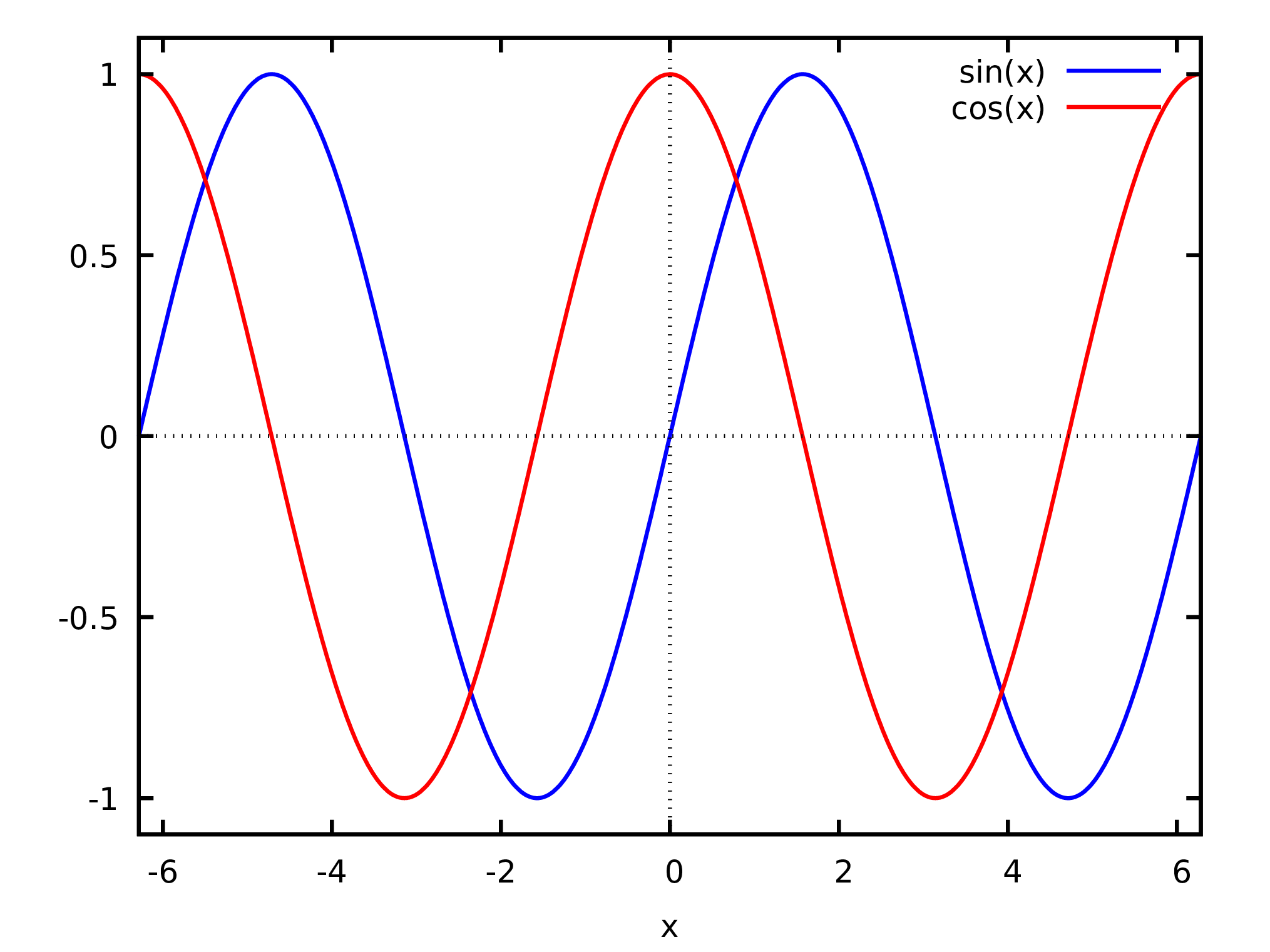
To plot several functions in the same window, those functions must be placed inside a list. For instance, the following command shows the plots of functions sine and co-sine.

(%i77) plot2d ( [sin(x), cos(x)], [x, -2*%pi, 2*%pi])$

**Figure 4:** Plot of functions sin and cosine.

It would be enough to simply give the names of the functions, as in [sin, cos]. Provided they are functions of only one variable, plot2d will input into them the values of the variable, within its interval defined by [x, -2*%pi, 2*%pi].

The resulting plot is shown in Figure 4. In the cases when you would like to plot functions that you defined, it is more fool-proof to just give the name of the function, making sure that it depends on only one input variable. In the cases when your function $f (x)$ gives as result an algebraic expression on $x$ , it is equivalent to use $f (x)$ or $f$ ; but in the cases when $f (x)$ does not result in an algebraic expression of $x$ , that will fail.

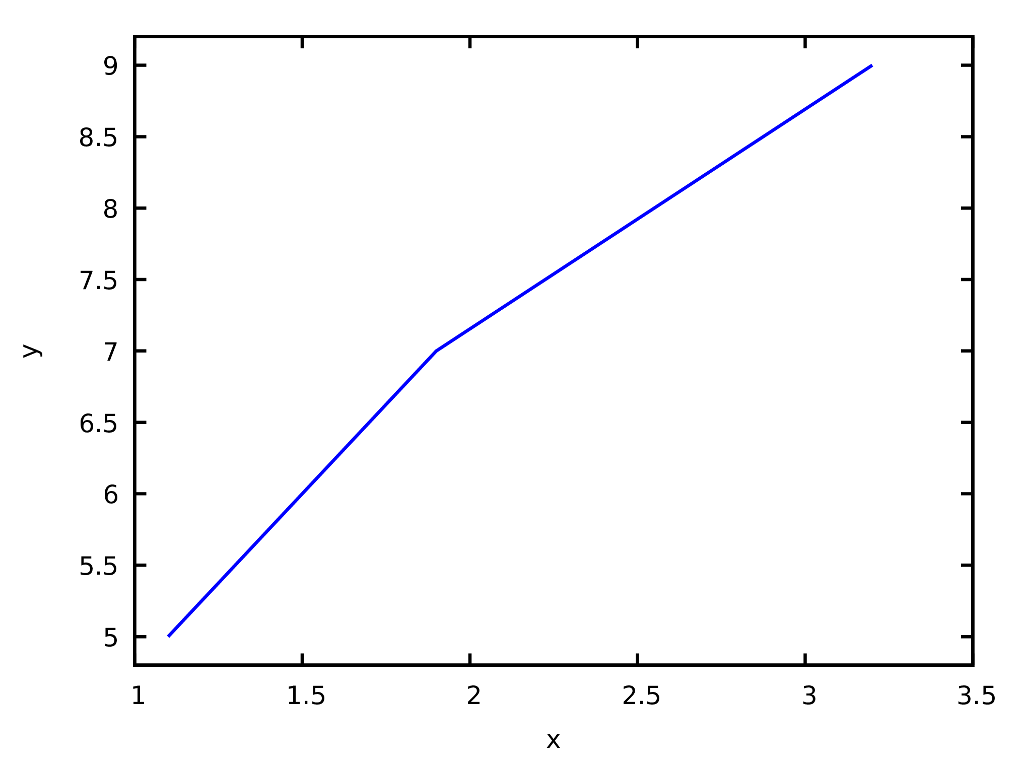
To show several points in a plot, the coordinates of the points can be given as lists, within another, with lists of points in a two-coordinate system. The two coordinates of each point can be given as a list, inside another list with all the points. For example, to show the three points (1.1, 5), (1.9, 7) and (3.2,9) in a plot, the points coordinates can be placed inside a list linked to the symbol p:

(%i78) p: [[1.1, 5], [1.9, 7], [3.2, 9]]$

To create the plot, it is necessary to give plot2d a list that starts with the keyword discrete, followed by the list of points. In this case it is not mandatory to specify an interval of values for the variable in the horizontal axis:

(%i79) plot2d ([discrete, p])$

**Figure 5:** Plot of a line defined by three points.

The plot is shown in Figure 5. By default, the points are linked by line segments; to show only the points, without line segments, the option [style, points] is used.

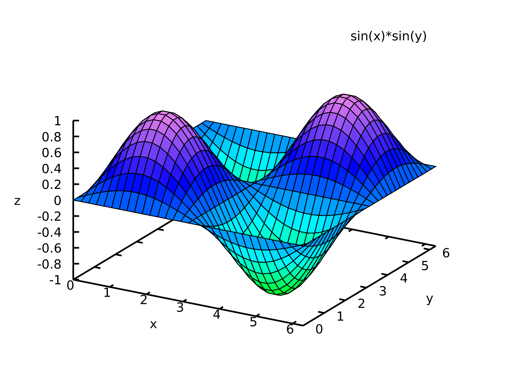
Command plot3d is used to plot functions of two variables. For example, the following command creates the plot shown in Figure 6:

(%i80) plot3d ( sin(x)*sin(y), [x, 0, 2*%pi], [y, 0, 2*%pi])$

**Figure 6:** Plot of function $\sin (x) \sin (y)$ .

Moving the mouse over the plot, while its left-side button is pressed, the surface will be rotated showing how it looks from different sides. The command plot3d also accepts a list of several functions to be plotted in the same window. It is also possible to give a list o 3 functions of 2 parameters, that define the 3 components of a position vector that describes a surface (parametric plot).

Both plot2d and plot3d accept the options pdf_file, png_file and ps_file which are used to save the plot into a file in PDF, PNG or PostScript format. For instance, the following command saves the plot produced by command (%i74) into a PNG file:

(%i81) plot2d ([sin, cos], [x,-2*%pi,2*%pi], [png_file,"./plot1.png"]);

(%o81)                      [./plot1.png]

The command does not show the plot but shows a list with the file created, in this case a PNG file. The initial characters "./" indicate that the file named "plot1.png" is located in the current directory where Maxima is running. If you don't give any initial characters "./" and you finished the plot2d command with a semicolon, the output will show you in which directory the file was placed, in a default directory.

There are many other options for plot2d and plot3d, as well as other graphic functions, which are explained in the Maxima manual.

14 Functions

In Maxima what is usually referred to as a function is a program with some input arguments and an output. Those functions can be defined using Maxima's syntax or using Lisp commands. It is even possible to redefine any of the functions mentioned in previous sections; for instance, if in the Maxima version being used some function has a bug that has already been fixed in a more recent version, it is possible to load the new version of the function and, unless it introduces conflicts with other older functions, it should work correctly.

Maxima functions are normally called by giving their name followed by its input inside parenthesis, as in diff(cos(x),x). Functions with only one input argument can also be defined to be used just by giving their name before or after their argument, as in 34! which computes the factorial of 34; the name of the function is ! and 34 is its input argument (see documentation for prefix and potfix). And functions of two input arguments can be defined to be used by just giving their name in between the two arguments, as in 3*7 (see documentation for infix).

As a first example, let us create our own version of the factorial function, which we will name fact:

(%i82) fact(n) := if n <= 1 then 1 else n*fact(n-1);

(%o82)       fact(n) := if n <= 1 then 1 else n fact(n - 1)


(%i83) fact(6);

(%o83)                            720

It is not necessary to use any command to return the output, since the output of the last command in the function will become the output of the function. A function can call itself recursively as it has been done in this example.

Several Maxima commands can be grouped together by placing them inside parenthesis and separating them by commas. Those commands are run sequentially and the result of the last command will be the result of the whole group. Each command can be indented and can expand more than one line. The following example defines a function that adds all the arguments given to it:

(%i84) add([v]) := block([s: 0],
                          for i:1 thru length(v) do
                             (s : s + v[i]),
                             s)$

(%i85) add (45,2^3);

(%o85)                             53


(%i86) add (3,log(x),5+x);

(%o86)                       log(x) + x + 8

A list was used as the argument for the function, which makes the function accept any number of input parameters (or none) and all the arguments given will be placed in a list linked to the local symbol v. Function block was used to define another local symbol s, initially linked to the value 0, which by the end of the function will be linked to the sum of the input variables. The first element given to block must be a list, with the names of symbols that are to be considered local to the function, each one with or without an initial value, and the remaining commands after that list define the function. The function for iterates the local variable i ---in this case from 1 up to the length of the list--- with increments, by default, equal to 1 (option step can be given to modify the default value of that increment). After the for loop, we gave the name of variable s, to make it become the output of the function.

When an unknown function is used no errors are triggered; instead, the unknown function is echoed in the output; for example:

(%i87) 2*4*maximum(3,5,2);

(%o87)                     8 maximum(3, 5, 2)

Most of Maxima functions behave the same way when they fail to give a result. For instance,

(%i88) log(x^2+3+x);

                                 2
(%o88)                      log(x  + x + 3)

That behavior is very useful, because it makes it possible to change the value of the arguments later on and to reevaluate the function. For example, substituting the symbol x in this last result by the floating-point number 2.0, the logarithm would then be computed and its numerical value shown:

(%i89) subst (x=2.0, %);

(%o89)                           2.197